Advanced On-Chip Linearization in the A1335 Angle Sensor IC
By Alihusain Sirohiwala and Wade Bussing,
Allegro MicroSystems, LLC
Introduction
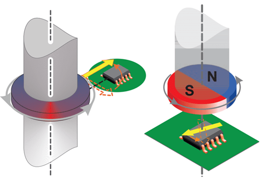
Numerous applications in industries—spanning from industrial automation and robotics, to electronic power steering and motor position sensing—require monitoring the angle of a rotating shaft either in an on-axis or off-axis arrangement.
The design of any successful angle measurement system for the above applications must be based on the needs of the particular application. These include: arrangement (off-axis or on-axis), air gap, accuracy, and temperature range, among others.
A magnetic angle measurement system has two main sources of error:
Sensor IC related errors:
- intrinsic nonlinearity;
- parametric temperature drift;
- noise.
Magnetic input related errors:
- field strength variation;
- field nonlinearity.
Each Allegro angle sensor IC is tested and calibrated during production at Allegro using a homogenous magnetic field. As a result, intrinsic IC nonlinearity and temperature drift are reduced to a minimum before the angle sensor IC is shipped to customers. Please refer to product datasheets for temperature drift information.
When using a magnet in a design, the magnetic input will most likely not be homogenous over the entire range of rotation—it will have inherent errors. These magnetic input errors cause measurement error in the system.
These factors become especially important when considering side-shaft or off-axis designs that have higher intrinsic magnetic errors. Even the most accurately calibrated angle sensor IC will produce inaccurate results if the error contribution from the magnetic input dominates. In most cases, even on-axis magnetic
designs suffer from relatively large misalignments that occur during the assembly of the customer module in the production line. These magnetic error sources are inevitable and mitigating them is almost always expensive and often impossible.
The approach of the Allegro A1335 angle sensor IC is to solve this problem by using advanced linearization techniques to compensate for these errors at the customer’s end-of-line manufacturing location.
This document shows how magnetic-input-related errors in excess of ±20 degrees can be linearized by the A1335 to as low as ±0.3 degrees—roughly a 65× improvement.
This linearization can be performed based on data from a single rotation of the target magnet around the angle sensor IC. The angle readings from this rotation are used to generate linearization coefficients which can then be stored into on-chip EEPROM, optimizing that angle sensor IC, for that magnetic system. Allegro can provide the necessary software and/or DLLs to help customers program these devices at their end-of-line.
Linearization Options
There are two linearization techniques offered in the A1335 angle sensor IC. The first is called segmented linearization, and the second is called harmonic linearization.
Segmented linearization is a programmable feature that allows adjustment of the transfer characteristic of the angle sensor IC such that linear changes in the applied magnetic field vector angle can be output as corresponding linear angle increments by the angle sensor IC. It is performed on the data collected from one rotation of the magnet around the angle sensor IC.
On the other hand, harmonic linearization applies linearization in the form of 11 correction harmonics whose phase and amplitude are determined by means of an FFT (fast Fourier transform) performed on the data collected from one rotation of the magnet around the angle sensor IC. Both of these techniques can be readily implemented using Allegro-provided software to calculate coefficients and program on-chip EEPROM. Contact your local Allegro representative to obtain the latest DLLs, software GUIs, and programming hardware.
Definitions
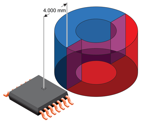
AIR GAP
Two different air gap definitions can be used when discussing about magnetic field sensors: package air gap and crystal air gap.
PACKAGE AIR GAP
Package air gap is defined as the distance between the nearest edge of the sensor housing and the nearest face/tangent-plane of the magnet.
CRYSTAL AIR GAP
Crystal air gap is defined as distance between the sensing element in the sensor housing and the nearest face of the magnet.
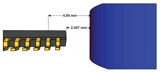
To illustrate this difference, Figure 2 shows both the crystal air gap (4.0 mm) and package air gap (2.407 mm) for an A1335 angle sensor IC and magnet in a side-shaft or off-axis configuration.
In this document, the term air gap always refers to the package air gap, unless otherwise stated. The sensing elements are 0.36 mm below the top surface of the package. The distance between the sensing element center and the closest short edge of the package is 1.593 mm.
ANGLE ERROR
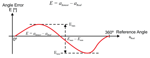
Angle error is the difference between the actual position of the magnet and the position of the magnet as measured by the angle sensor IC. This measurement is done by reading the angle sensor IC output and comparing it with a high resolution encoder (refer to Figure 3).
ACCURACY ERROR
Further down in this document, the angle error is displayed as a function of misalignment. For that purpose, it is necessary to introduce a single angle error definition for a full rotation. The ‘summarized’ angle error on one full rotation is defined as angular accuracy error, and it is calculated according to the following formula:
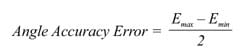
In other words, it is the amplitude of the deviation from a perfect straight line between 0 and 360 degrees.
It is important to distinguish between angle sensor IC related errors and magnetic input related errors. This document highlights how advanced features in the A1335 angle sensor IC can be used to compensate for magnetic input related errors.
As far as angle sensor IC related errors are concerned, intrinsic nonlinearity and parametric temperature drift are optimized for each Allegro angle sensor IC at Allegro’s end-of-line test operation (see datasheet specifications for those parameters) before shipping to the customer. Noise performance can be optimized
for the customer application by using on-chip filtering (see ORATE settings in A1335 Programming Manual).
Magnets
In order to compare the performance of the segmented or the harmonic linearization options, both linearization techniques were performed on the same magnets. The magnets used were Neodymium N45 dipole ring magnets available from Super Magnets. Figure 4 and Figure 5 illustrate magnet dimensions.

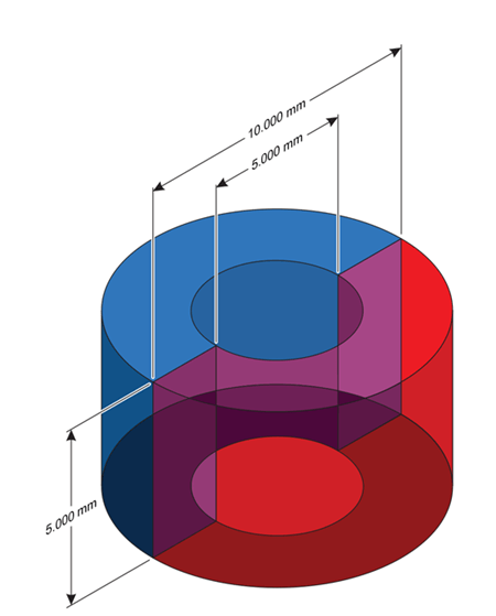
Table 1: Off Axis (Left) and On Axis (Right)
| Magnet Name | Manufacturer | Inner Diameter |
Outer Diameter |
Height | Material |
| R1 | Super Magnets | 7 mm | 10 mm | 3 mm | N45 Ni Plated |
| R2 | Super Magnets |
5 mm | 10 mm | 3 mm | N45 Ni Plated |
Average Magnetic Field and Air Gap Dependency
The first step in the system design is to choose an appropriate magnet for the application air gap. Usually the air gap is in a range from 2 to 4 mm. Figure 5 shows the magnetic field as a function of air gap for the magnets R1 and R2.
By default, many Allegro angle sensor ICs are trimmed to datasheet specification at 300 G (30 mT). In the case of the A1335, there is also a magnetic autoscaling feature that dynamically adjusts internal gains to compensate for dynamic variations in air gap. However, care should be taken with the magnetic design so that the air gap variation does not result in fields that are too low (inadequate signal to noise ratio) or too high (saturation of signal-chain blocks). In general, field strengths from 300 G to 1000 G are ideal, with improved noise performance at the higher field levels.
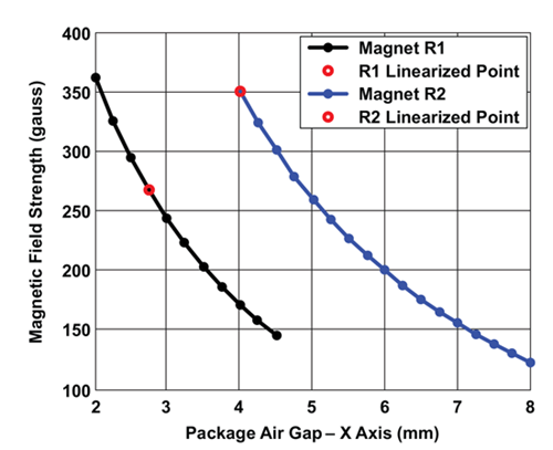
Magnitude VS Air-gap
As Measured by A1332, for Magnets R1 and R2
Magnet Error Analysis
Using Magnets R1 and R2, an analysis was performed of the inherent nonlinearity observed in the magnetic signal when measuring angle. Measurements were taken using a calibrated A1332, the predecessor to the A1335, under ideal alignment as shown in Figures 7 and 8.
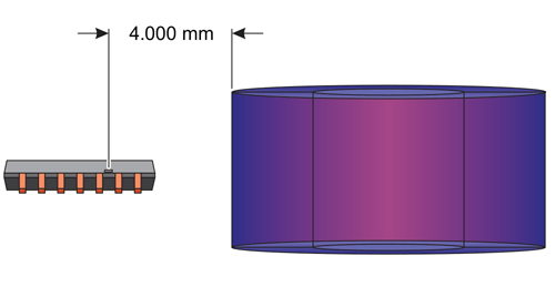
Side-View
Based on one rotation sampling the angle sensor IC output at equidistant angular points, the transfer characteristic as shown in Figure 9 is obtained.
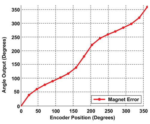
Analyzing the above angle error in the frequency domain with an FFT, the error versus harmonics as shown below in Figure 10 is obtained.
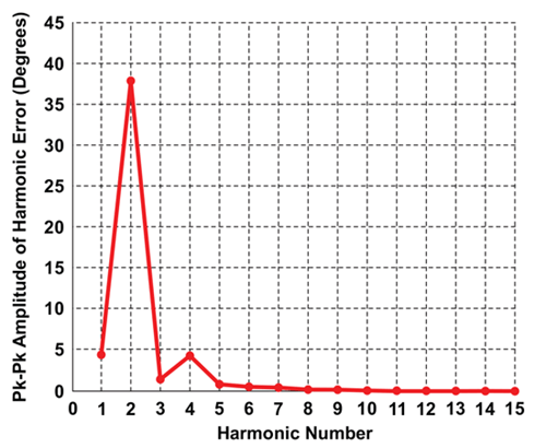
Magnet R1
Figure 11 shows a similar analysis on magnet R2.
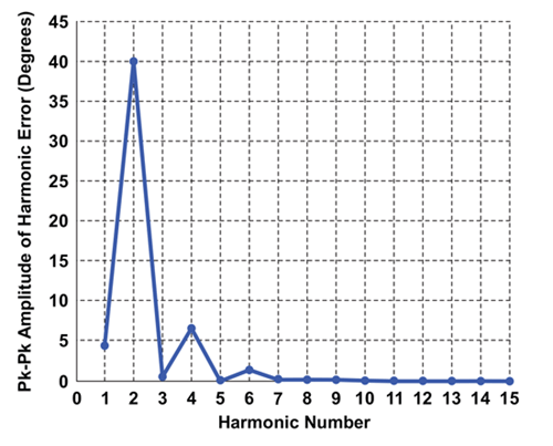
Magnet R2
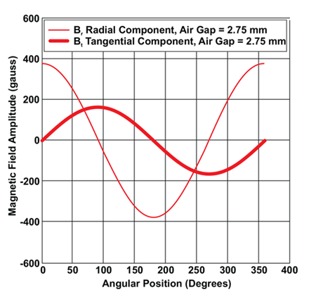
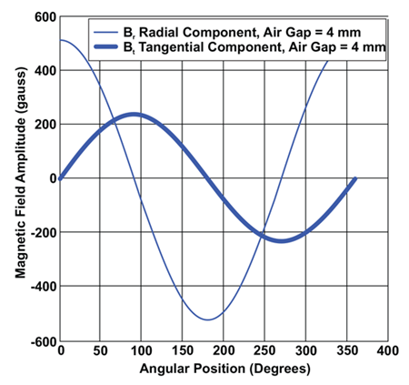
It is clear from the FFT data that most of the inherent error in both magnets R1 and R2 is from 2nd harmonic contributions, whereas 1st, 4th, 3rd and higher harmonics are responsible for the remainder of the error. The root cause of this error is a mismatch in the amplitude of the radial (Br) and tangential (Bt) components. The magnetic field vector, whose phase or angle is being measured by the angle sensor IC, can be expressed as two orthogonal components Br and Bt as shown in Figure 12.
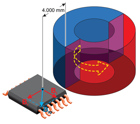
of the Field
Ideally, these components should be identical in amplitude, and orthogonal in phase. Any deviation from this ideality introduces error in the resultant angle measurement. In ring magnets for side-shaft sensing, the mismatch in the radial and tangential component is inherent to the magnet design and manufacturing process and can vary depending on the manufacturer, and the manufacturing method. In the case of cylindrical magnets, the radial and tangential mismatch can be introduced by adding eccentricity or misalignment between the angle sensor IC and magnet.
These mismatches result in an angle error profile with terms at multiple harmonics. Therefore, it is clear, that only correcting for the 2nd harmonic error term will not be sufficient, especially if high-accuracy performance is required.
Components
Components
Segmented Linearization
The A1335 Segmented Linearization is a programmable feature that allows adjustment of the transfer characteristic of the device so that changes in the applied magnetic field can be output as corresponding linear increments.
Linearization
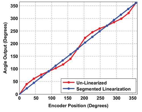
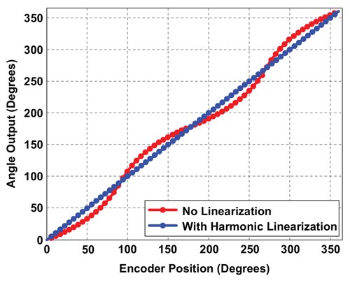
Figure 15, above illustrates the angle output of the A1332 both with and without the Segmented Linearization.
In order to achieve this, an initial set of linearization coefficients has to be created. The user takes 15 samples of angle: at every 1/16 interval of the full rotational range from 0 to 360 degrees. The zero-reference point is set by the LIN_OFFSET EEPROM field. This becomes the zero-error point, and is therefore not represented
in the coefficient table. Likewise, the 360-degree point is identical to the zero-reference point and is also not represented in the coefficient table. The rest of measured angles at the segment boundaries are placed in the LIN_COEFF1 ... LIN_COEFF15 EEPROM fields. The following instructions describe the basic algorithm for applying these linearization coefficients. Sample implementations of this method are available through Allegro Customer Evaluation Software Tools. Figure 15 shows the Angle
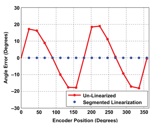
output versus an Encoder reference, both with and without Segmented Linearization applied. Figure 16 shows the Angle Error by subtracting the reference encoder value, both with and without Segmented Linearization applied. Figure 17 shows a zoomed-in look at the Angle Error profile with Segmented Linearization applied.
Steps for Implementing Segmented Linearization
- Collect data
Turn off all post-linearization algorithmic processing; this includes ZeroOffset, Post Linerization rotation (RO), Short Stroke Inversion (IV), and the Rotate Die bit (RD). Prelinearization adjustments may be left on, such as ORATE settings, IIR filter (FI), and prelinearization rotation (LR).
Enable segmented linearization by setting the SL to 1 (SL bit in CFG_2, word 6, EEPROM bit 16, SRAM bit 20). Turn on Segmented Linearization Bypass bit (SB bit, word 6, EEPROM bit 21, SRAM bit 25). This allows measurements to be taken without otherwise applying the linearization coefficients.
Find the desired zero-reference point, realizing that the linearly interpolated segments will be +22.5, +45.0, etc. from this reference point. For side-shaft, picking a point where the error is at a peak or valley is optimal. The angle sensor IC reading at that point will be entered into the LIN_OFFSET coefficient in the next step.
Move the encoder in the direction of increasing angle position. If the sensor angle output does not also increase, then either set the LR bit to reverse the direction of the angle sensor IC, or rotate the encoder in opposite direction for this calibration step. (In which case the post-linearization rotate bit (RO) will likely need to be set after calibration is complete). See A1335 programming reference for more details.
Move in encoder steps of 22.5 degrees and read 15 angle sets.This process will produce the 15 LIN_COEFF coefficients.
- Program Coefficients
Program LIN_OFFSET after multiplying with * (4096/360), written in HEX after rescale.
Program each of LIN_COEFF after multiplying with *(4096/360), written in HEX after rescale.
- Enable Linearization
Set EEPROM bit SB=0, since it is no longer needed to bypass the linearization function (data collection in step 1 is already completed). Set EEPROM bit SL = 1 (note: it should already be set to 1 from step 1), to enable segmented linearization. The angle sensor IC output should now linearly interpolate along each segment and produce a corrected angle output.
Results
Figure 16 illustrates the segmented linearization performance in the form of angle error compared to a known-good encoder angle reference.
Linearization
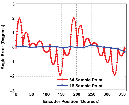
Although accurate as shown, Figure 16 is not a very insightful depiction of the true angle error performance. It only shows the angle error at the points in the transfer function where the postlinearization error is the least. If the same device were to be measured again, with a much smaller angle step between samples, the result would be what is shown in Figure 17. Notice the “lobes” of error between successive linearization points. These are expected since in each segment, the error is approximated as a straight line, when in fact it is sinusoidal. Given this type of sinusoidal input error pattern, Figure 17 is about the best performance that can be achieved with a segmented approach using 16 segments.
The segmented linearization implemented in the A1335 only allows for this 16-segment linearization. The performance of this method could conceivably be improved by either increasing the number of segments or by making the segment length variable, so that finer segments can be used for areas with higher curvature.
However, both of these enhancements result in higher processing time and complexity.
Resolution, Segmented Linearization
Harmonic Linearization
As seen in the section, analyzing errors from magnets R1 and R2, it is clear that these errors are sinusoidal in nature, meaning that they can usually be well described by constituent harmonics of appropriate phase and amplitude. Harmonic Linearization takes advantage of this property and applies the linearization in the form of 11 harmonics whose phase and amplitude are determined by means of an FFT (Fast Fourier Transform) performed on the data collected from one rotation of the magnet around the angle sensor IC at the customer’s end-of-line.
Linearization
There is a great deal of flexibility built into the Harmonic Linearization function. The value of the individual harmonic Amplitudes and Phases are stored in 12-bit EEPROM fields for each of 11 harmonics.
The number of harmonics that need to be applied in a linearization can be specified by the user using the 4-bit HAR_MAX EEPROM field. This setting determines how many individual harmonic components (from 1 to 11) are used for computing harmonic linearization. (The Adv fields are used to determine which harmonics are applied for each component.)
The 2-bit Field ‘Adv’ field sets the increment between sequential pairs of applied harmonic components. The value entered, n (in the range 0 to 3), indicates how many harmonics to be skipped from the previous component to the current component. The count is applied as 1 + n. For example, the first component (0x0C) minimum (n = 0) is the 1st harmonic and the maximum (n = 3) is the 4th harmonic. The effect is cumulative; when all components are set to n = 3, the 44th harmonic is available at the fifteenth component (0x16). As an example, a magnet R1 is used in a side-shaft configuration in order to linearize a sensor.
In addition to enabling side-shaft applications, the flexibility built into this linearization method is also very useful in removing static misalignment errors at the customer’s end-of-line.
Steps for Implementing Harmonic Linearization
- Collect data
Turn off all post-linearization algorithmic processing; this includes ZeroOffset, Post Linerization rotation(RO), Short Stroke Inversion (IV), and the Rotate Die bit (RD). Prelineariztion adjustments may be left on, such as ORATE settings, IIR filter (FI), and pre-linearization rotation (LR).
Move the encoder in the direction of increasing angle position. If the angle sensor IC does not also increase, then either set the LR bit to reverse the direction of the angle sensor IC, or rotate the encoder in opposite direction for calibration (in which case the post-linearization rotate bit (RO) will likely need to be set). See A1335 programming reference for more details.
Move in encoder steps such that the resultant data is a power of 2. Usually, 32, or 64 evenly spaced data points are sufficient.
- Program Coefficients
Perform an FFT on the measured data and then program HARMONIC_AMPLITUDE, HARMONIC_PHASE, ADV, and HAR_MAX fields based the preferred implementation. A sample implementation of these features is available from your Allegro representative.
- Enable Linearization
Set EEPROM bit HL=1 to enable Harmonic linearization. The sensor output should now produce a corrected angle output.
Results
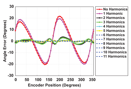
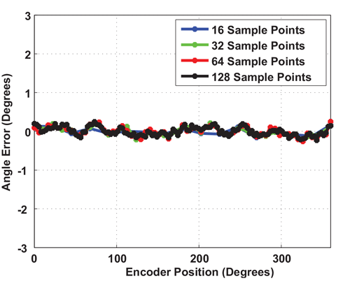
Figure 19 shows Harmonic Linearization performance for magnet R1, with HARMAX = 1 through 11 (and all ADV fields = 0) as measured on an A1332. (And all ADV fields = 0). In other words, this shows the performance as harmonic correction is incrementally applied from the 1st up to the 11th harmonic.
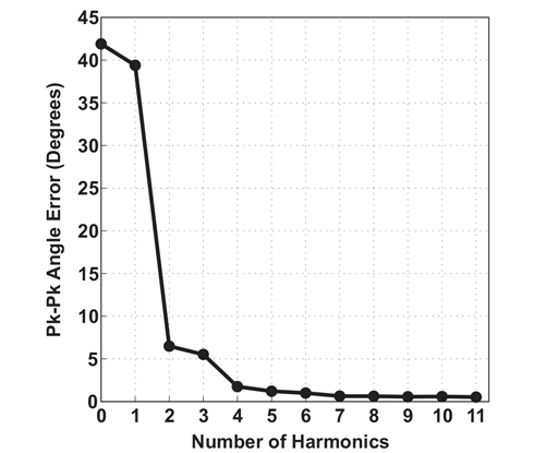
The same result is summarized in Figure 20 to show the pk-pk angle error (on the y axis) versus the number of correction harmonics applied. The sharp drop in angle error after the 2nd harmonic correction is expected since the majority of the spectral error content resides in the 2nd harmonic (see section analyzing magnetic errors).
In order to further investigate the error performance with harmonic linearization applied, especially when using small angular steps, the same device was re-measured several times, with finer angle steps (higher resolution) with each run. The data shows no underlying higher error regions. The post-linearization error is sub-0.3 degrees.
as measured with an A1332
with HARMAX = (1 to 11), using R1
Harmonics Applied, using R1,
as measured with an A1332
Resolution, And Harmonic Linearization
Angle Latency Considerations
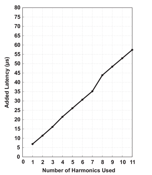
Both Segmented and Harmonic Linearization techniques are well-suited for on-axis and off-axis magnetic applications. While segmented linearization divides the magnetic range into smaller sections which are linearized in a piece-wise fashion, harmonic linearization allows for a sinusoidal-based compensation of the error signal, which helps remove the high harmonic error content in misaligned as well as side-shaft arrangements. The added performance from harmonic linearization comes at the cost of higher computation time. Figure 22 describes the added latency to the angle measurement, from each additional harmonic that is added to the harmonic linearization. For example, based on the data in Figure 20, it is clear that to achieve <1 degree, at least 7 harmonics of correction are needed. Now, looking at the added latency in processing time associated with 7 harmonics in Figure 20, it is 35 μs. This means that every angle sample will take an additional 35 μs to process. In contrast, the segmented linearization requires an additional computation time of 22 μs. Therefore, for this particular magnet, the improved error performance of
harmonic linearization comes at a cost of an additional 13 μs of latency. For many applications, the additional latency will not be a problem. As an example, in typical Electronic Power Steering (EPS) system hand-wheel angle sensor ICs, a new Angle value is requested every 1 ms, meaning that there is more than enough time to perform even 11 harmonics of linearization. Also, a lot of systems will avail of the ORATE feature of the A1335 in order to reduce the noise-floor of the angle measurement by oversampling. This will also inherently provide enough time to perform linearization functions without added latency since the additional averaging with allow for more time to be budgeted for linearization operations.
Harmonics Used
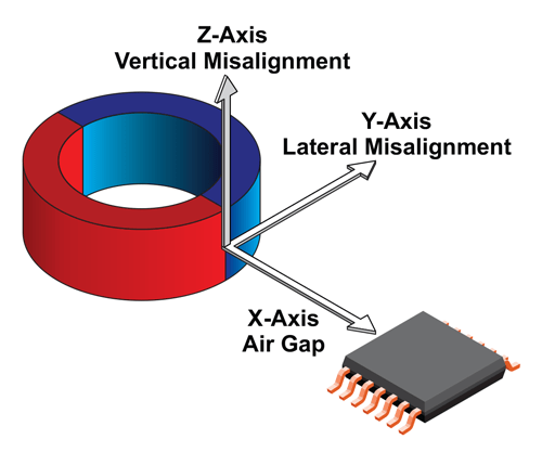
Effect of XYZ Misalignment on Linearized Angle Sensor IC
In this section, we analyze the performance of an angle sensor IC that has been linearized for magnets R1 and R2, and then mapped for misalignment errors in the X, Y, and Z axes as shown in Figure 23. In the case of both magnets R1 and R2, we use an initial starting position at X (air gap) = 2.75 mm and 4 mm respectively, with Y, Z = 0 mm, such that the angle sensor IC is positioned in the middle of the magnet height. We use this position as our Cartesian origin, and map misalignment performance from this reference according to the Table 2. The following data was collected using an Allegro A1332 angle sensor; A1335 performance will be similar or better.
Table 2: Mapping Range and Linearization Points for both Magnets R1 and R2
| Magnet R1 Axes |
Min (mm) |
Linearization Point (mm) |
Max (mm) |
| X (Air gap) | 2.0 | 2.75 | 4.5 |
| Y (Lateral) | -2.0 | 0.0 | 2.0 |
| Z (Vertical) | -2.0 | 0.0 | 3.0 |
| Magnet R2 Axes |
Min (mm) |
Linearization Point (mm) |
Max (mm) |
| X (Air gap) | 4.0 | 4.0 | 8.0 |
| Y (Lateral) | -2.0 | 0.0 | 2.0 |
| Z (Vertical) | -2.0 | 0.0 | 3.0 |
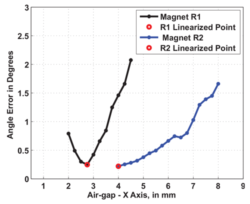
The angle error performance for both Magnets R1 and R2, as a function of air gap (X axis) is illustrated in Figure 24.
and R2
A few observations can be made by studying the plot in Figure 24. From the value of the angle error at the linearization point (denoted by the red circle), it is clear that the angle sensor IC is able to achieve very similar post-linearization performance for both magnets. From that limited perspective, both magnets can be used to achieve identical performance. However, upon studying the shape of the error curves versus air gap in Figure 24, it is clear that magnet R1 (black trace) has a steeper rise in error as the angle sensor IC is misaligned away from the linearization point (red circle), as compared to magnet R2 (blue trace).
As an example, increasing the air gap between the angle sensor IC and magnet R1 by 1 mm results in the about the same performance degradation as increasing the air gap between the same angle sensor IC and magnet R2 by 4 mm. The better air gap performance of magnet R2 can be attributed to the fact that it is a thicker ring magnet (5 mm thick) as compared to R1 (3 mm thick).
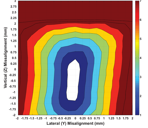
(Vertical and Lateral Axes) at Air Gap = 2.75 mm
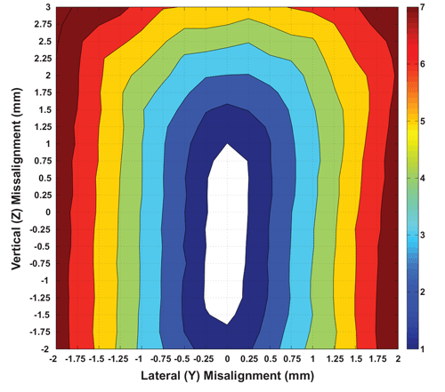
(Vertical and Lateral Axes) at Air Gap = 4 mm
In a similar fashion, the misalignment performance can be analyzed in both the lateral and vertical (Y and Z) axes by comparing the two filled contour plots for magnets R1 and R2, shown in Figure 25 and Figure 26 respectively. These plots have been generated by using the data from lab measurements mapping the performance at each point in space. For both these plots, the origin (Y = 0, Z = 0) position represents the performance at the linearized point (the same as the red dots in Figure 24). As the angle sensor IC is misaligned from this origin, the angle error observed at each point is placed in a color “bin” according to the legend shown. The numbers on the legend represent degrees of peak error. As an example, the white region in the middle of each plot denotes the area for which the angle error performance remains below ±1 degree. Similarly, the brown areas in each plot denote regions where the angle error is greater than ±7 degrees.
Looking at the two contour plots, it is clear that for the same misalignment in Y and Z, the angle sensor IC + magnet R2 combination result is lower angle error increase, as compared to angle sensor IC + magnet R1. As an example, the white area for which the angle error is less than ±1 degree is 0.669 mm2 for magnet R1 while it is 1.10 mm2 for magnet R2. Additionally, it is clear that the white area is vertically “elongated” for the case of R2, as compared to R1. This makes sense considering that the vertical height of ring magnet R2 (5 mm) is greater than that of ring magnet R1 (3 mm). These contours show the dependence of angle error performance on magnet geometry.
Conclusion
There are many factors involved in a successful angle sensing application. Minimizing angle error over temperature, positional misalignment, and air gap, is key. These variables are related to system-level design choices like magnet geometry, magnet arrangement (on-axis or off-axis), magnetic material, and mechanical tolerances. As such, flexibility is required of the angle sensor IC to work around these potential error sources without adding complexity and cost to the system-level design. Even the best magnetic angle sensor IC is only as good as the magnetic field that is senses.
On-chip, programmable, and customizable linearization, as implemented in the A1335 angle sensor IC, allows the system designer to meet the aforementioned accuracy objectives without adding additional complexity and cost to the system design.
The A1335 offers two linearization options—segmented and harmonic. Both of these options were studied using reference magnets R1 and R2. The results showed that although segmented linearization achieves faster processing times, it is limited in its ability to correct for sinusoidal error terms. In that regard, the harmonic linearization performs better. Additionally, the flexibility in the harmonic linearization, particularly the ability to change the number of correction harmonics used, allows the user to achieve the optimal trade-off between computation time and error performance. For both magnets R1 and R2, it was seen that ±20 degrees of angle error can be brought to within ±0.3 degrees with linearization applied.
Lastly, using the mapping technique, the effect of mechanical misalignment of the linearized angle sensor IC was studied. It was seen that a taller ring magnet translates into better tolerance to vertical misalignments, whereas a thicker ring magnet translates into better tolerance to changes in air gap.
Whatever the angle sensing challenges faced by the system-level designer, a combination of appropriate magnetic design and advanced on-chip linearization in the Allegro A1335 can help achieve the desired performance while minimizing added complexity and cost.