Microcontroller-Based Linearization of Angular Sensor ICs
Introduction
Magnetic angle sensors are often a good choice for fast, reliable, contactless measurement of the angular position of a system, especially in dirty environments where optical encoders may not be a good fit.
Allegro MicroSystems, LLC, offers a wide range of angular sensor ICs [1] for different applications. These sensor ICs can measure the angle of diametrically magnetized encoder magnets
in a side-shaft or end-of-shaft setup, as shown in Figure 1.
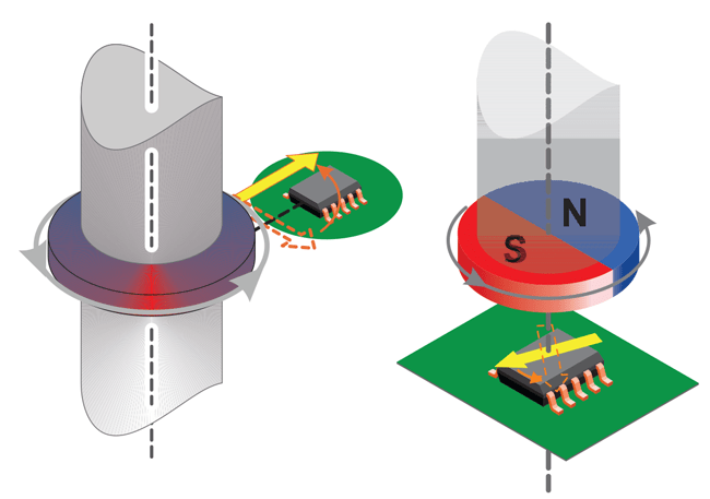
end-of-shaft angle measurement (right)
Measurement Errors
All Allegro angle sensor ICs are calibrated at final test in the factory using a homogenous magnetic field. This is done to minimize the native error of the sensor. However, especially in side-shaft applications, the magnetic field angle at the sensor transducer is not identical to the mechanical angle of the shaft that is to be measured. The main contributor to this difference is the shape of the magnetic field emitted from the encoder magnet.
Other sources of mismatch between mechanical and magnetic field angle are magnet misalignment, magnet imperfections, remaining sensor inaccuracy and drift, and thepresence of ferromagnetic materials.
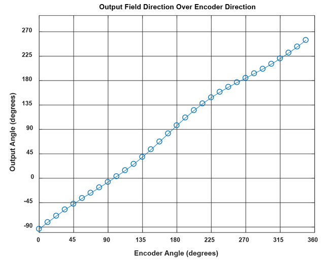
It can be concluded that all systems, and especially sideshaft-systems, suffer from a mismatch between the encoder angle and the measured angle. A typical transfer curve for a side-shaft application can be seen in Figure 2.
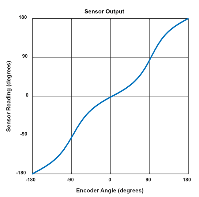
angle in a side-shaft setup
These measurement errors are called nonlinearities and can be compensated through a process called linearization.
Linearization
Some Allegro sensor ICs, such as the A1335, the AAS33001, and the AAS33051 have embedded logic that allows for the linearization of input data. However, other sensor ICs, such as the A1330, A1333, A1337, A1338, or A1339, do not have this functionality on chip. In cases where a sensor IC without the built-in functionality to linearize the data is used, external linearization using a microcontroller may be required to achieve the required accuracy in a particular application.
This application note will:
- Explain the fundamentals of linearization
- Show how to process real measured data to calculate correction data
- Detail three ways of storing the correction data
- Detail how to apply the correction
- Compare the accuracy of the proposed methods
Definitions
Encoder Angle
The angle reported by an accurate, high-resolution external encoder.
Sensor Angle
The angle reported by the angle sensor IC.
Angle Error
Angle error is the difference between the actual position of the magnet and the position of the magnet as measured by the angle sensor IC. This is calculated by subtracting the encoder angle from the sensor angle:
error = (α_sensor – α_encoder ) .
However, if the sensor angle is 359° and the encoder angle is 0°, the error should be –1° and not +359°. To wrap around any error outside of ±180°, the modulo operator can be used:
error = mod[(α_sensor – α_encoder) + 180,360] – 180.
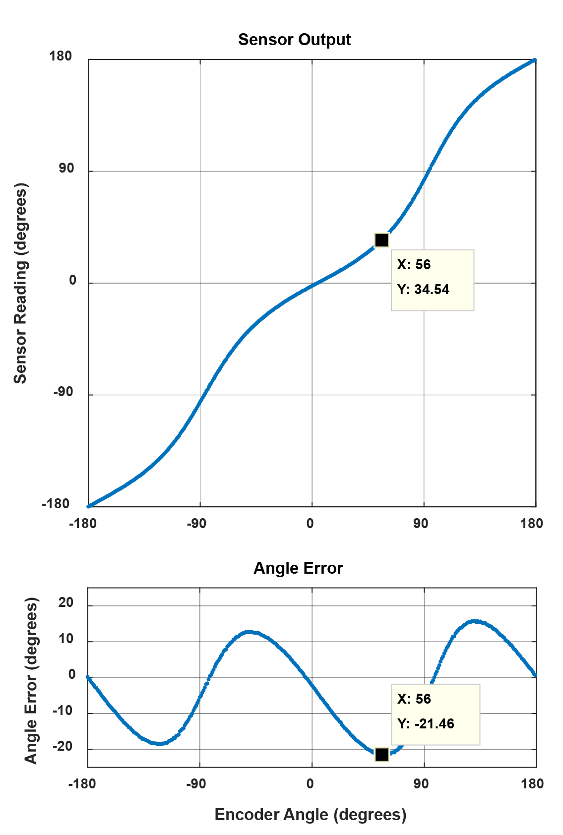
A sample plot of the angle error in a side-shaft application is given in Figure 3.
Maximum Absolute Angle Error
The maximum absolute angle error is the largest absolute difference between the actual position of the magnet and the position of the magnet as measured by the angle sensor IC over a full rotation.
In Figure 3, the maximum angle error is 21.46°, measured at an encoder angle of 56°.
Goal of Linearization
The goal of linearization is to determine, store, and apply a function that minimizes the measured sensor angle error as compared to the encoder angle value. This minimizes the difference between measured sensor angle and actual encoder angle.
This goal can be achieved in different ways. Three common techniques will be detailed in this applications note.
The techniques presented depend on a single calibration phase (typically performed at the customer’s end-of-line test), after which a fixed correction function is applied.
Prerequisites to Linearization
Prerequisites to linearization using the techniques detailed here are the following:
- During production, known angles need to be applied to the sensor system.
- During production, sensor angles need to be read out.
- The system to be linearized needs a microcontroller, to which linearization information is written during the production process and which performs linearization in the application.
Limits to Linearization
Linearization using the methods described here has some limits:
- Sensor noise will not be corrected by linearization.
- Any drift of the sensor after calibration will not be corrected.
- Changes in the mechanical system after calibration will not be corrected by linearization. A common example is dynamic change of magnet position due to vibrations and torque
- If the input positions during the calibration are not accurately recorded, the accuracy of the correction will be limited in the same way.
Linearization Method
1. Data Recording
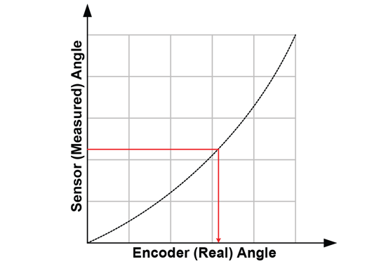
To generate the data needed for linearization, measure sensor output [y0 … yn] at known encoder angles [x0 … xn]. These encoder angles do not need to be equidistant, although it is common to use equidistant angles.
The recording of values is shown in Figure 5.

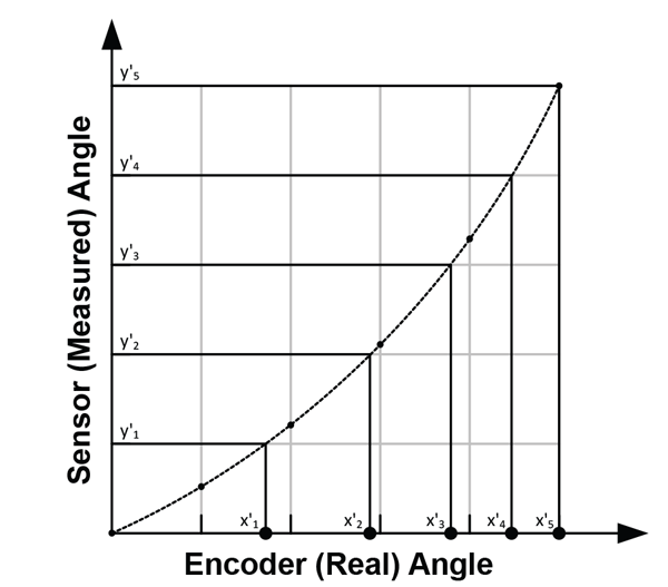
2. Coordinate Transformation to Sensor Angle As the correction function has to work based on the sensor data, the recorded data points should be transformed into the sensor coordinate system.
This means that instead of expressing the sensor angle as function of the real angle, it is required to express the real angle as function of the sensor angle. Therefore, sensor angles [y'0 … y'n] are chosen, for which corresponding encoder angles [x'0 … x'n] need to be determined. To do this, a fit needs to be applied through the data points. This can be done through spline interpolation, as shown in Figure 6.
3. Correction Curve Calculation
In order to create a function that converts the angle measured at the sensor into the encoder angle, correction values need to be calculated. These correction values are calculated as [c0 … cn] = [x'0 … x'n] – [y'0 … y'n].
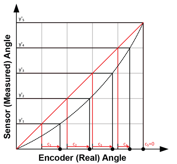
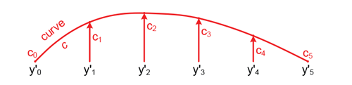
In the end, these values describe a correction curve, c, which gives the correction values as a function of the sensor angle. Figure 8 shows a plot of the curve c over sensor angle.
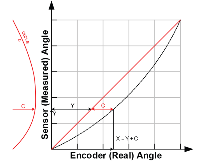
4. Correction Curve Application to Data
To apply the correction to a measured sensor data point, a correction value C for sensor data point Y needs to be calculated based on the correction curve c. This is graphically represented in
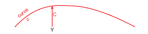
The correct angle value X is then determined as X = Y + C. This is graphically represented in Figure 10.
Correction Curve Storage Options
In this document, three ways to store the correction curve will be investigated. There are numerous other possibilities. However, the methods presented here service a wide range of needs while requiring modest implementation and calculation efforts. Of these methods, linear interpolation is hardware-implemented in the A1335, the AAS33001, and the AAS33051. Harmonic correction is implemented only in the A1335.
Harmonic Correction
The correction curve often has a periodic shape. By dissecting it into harmonics and storing the phase and amplitude of the harmonics, a compact storage is possible. This is clearly the case, for example, in Figure 3.
The advantage of harmonic correction is that only very few parameters need to be stored to correct the sensor data. The disadvantage is that the microcontroller needs to perform cosine calculation, which limits the speed.
Linear Interpolation
As a second method, it is possible to approximate the correction curve using a piecewise linear function.
This method requires more storage parameters to be used than harmonic correction, but takes less calculation time. The code size for the calculation method is also smaller.
Lookup Table
The third method to store the correction curve is to use a lookup table. This requires a large table in which the correction parameters are stored, but since the correction value can be taken directly from the lookup table, no interpolation steps are needed.
This keeps the linearization code very simple and fast.
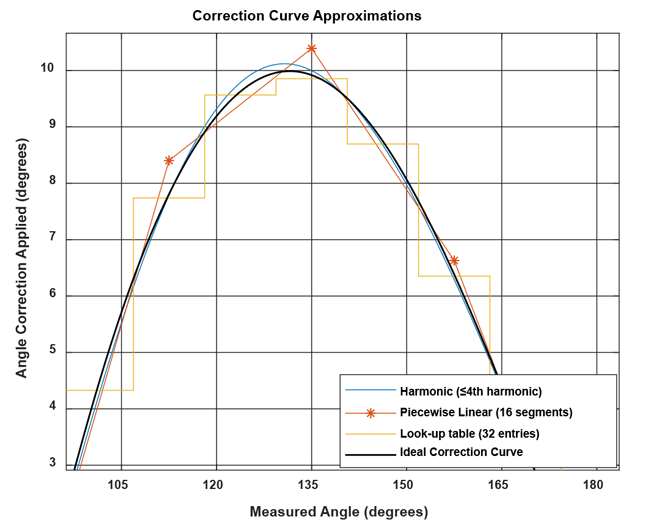
Correction Method Comparison
Figure 11 and Figure 12 show a comparison between the expected outputs obtained from the data in Figure 3 when the correction curve is stored as a harmonic approximation, piecewise linear interpolation, and lookup table.

Correction Curve Determination
The implementations in this document were implemented in MathWorks MATLAB™. As this is commercial software, licensing costs apply to using it, which may hinder use in production environments. A free software alternative to MATLAB is GNU Octave, which is available under the GNU GPLv3 license free of charge.
All functions used in this document are supported by both MATLAB and GNU Octave.
In these scripts, it is assumed that the sensor angle increases with increasing encoder angle. If this is not the case, the sensor angles must be inverted before proceeding with the other processing steps.
Sensor Output Capture
Initial data on the sensor angular output must be captured by the user. This is done by setting certain known angles, referred to as encoder angles in this document. Then the sensor angles are recorded. The sensor angles are the angles measured by the sensor. The number of points recorded can be more or less than the number of linear correction points. Recording more points, if
possible, is always better.
In general, recording at least 16 data points is enough for good correction performance in on-axis situations. In off-axis situations, at least 32 points are recommended.
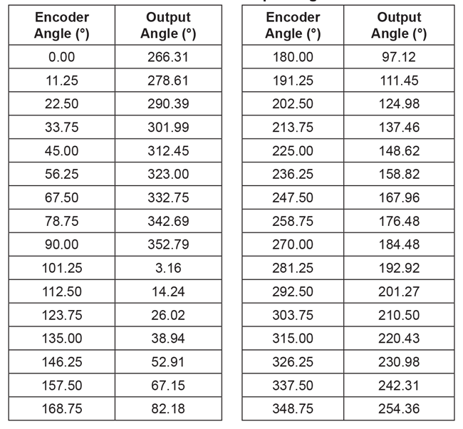
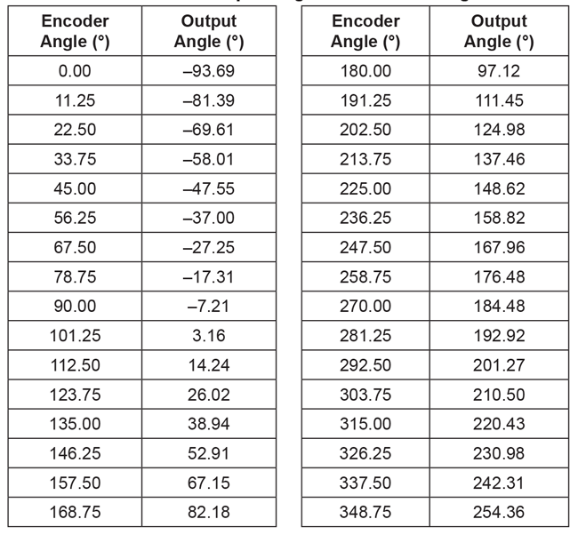
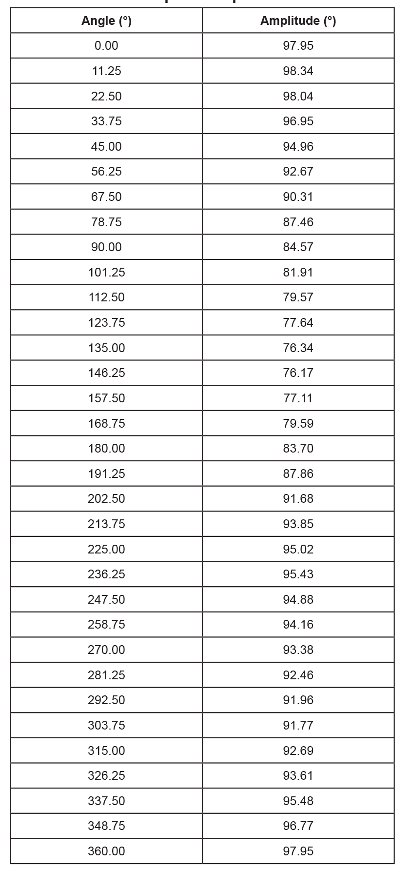
To apply piecewise linear correction with n segments (e.g. 32), recording at least n points will make good use of the available correction points. Recording about 2 × n points results in a nearly ideal performance. A real-life example of recorded points is given in Table 1.
Table 1: Recorded encoder and output angles
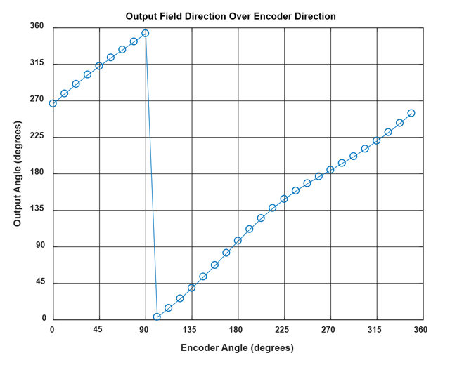
Sensor Output Overflow Removal
The jump in the sensor data around 100° input angle will cause difficulties in the next processing steps. It is removed by adding 360° to all values after the jump into negative direction. Also, the mean value of the data should be within ±180° to avoid other issues in later processing. This is achieved by the following lines:
    %% preprocessing

sensor_data_2 = sensor_data(:);

angle_input = angle_input(:);

% check if rising continuously with at most one overflow

if any(diff(sensor_data_2) == 0)

error('sensor data must be monotonously increasing')

elseif sum(diff(sensor_data_2) < 0 ) <= 1

% rising angle data with zero or one overflow, overflow will be corrected

sensor_data_2 = sensor_data_2(:) + 360*cumsum([false; diff(sensor_

data_2(:)) < 0 ]);

elseif sum(diff(sensor_data_2) < 0 ) > 1

error('only one data decrease permitted as overflow')

end

% correctly wrap around sensor data

rollovercorrection = round((mean(sensor_data_2) - 180)/360) * 360;

sensor_data_2 = sensor_data_2 - rollovercorrection;
The resulting values are shown in Table 2.
Table 2: Encoder and output angles after removing overflow
Data Replication
Eventually, correction data based on the sensor angles from 0° to 360° are needed. To avoid any edge effects, the sensor data will be replicated three times. This avoids edge effects in all cases by giving the possibility to always safely extract the values from sensor angle 360° to 720°.
    %extend sensor data

sensor_data_ext = [sensor_data_2(:); sensor_data_2(:)+360; ...

sensor_data_2(:)+720];

%extend input data

angle_input_ext = [angle_input(:); angle_input(:)+360; ...

angle_input(:)+720];
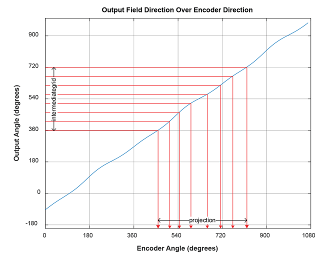
Projection onto Sensor Data Grid
In the next step, the encoder angle inputs corresponding to sensor outputs between 360° and 720° are calculated (called “intermediategrid” in the code below). This is done with 4096 steps, as a high resolution for this intermediate step benefits the final output quality.
    %% use spline to move the data from an ordered input grid

% onto an ordered output grid:

ordered_output_grid = 0:(360/4096):(360-360/4096);

intermediategrid = ordered_output_grid + 360;

projection = spline(sensor_data_ext, angle_input_ext, ...

intermediategrid);
This step is graphically illustrated in Figure 15.
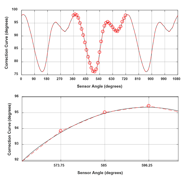
The difference between the angle encoder values and the sensor outputs is the correction curve and can be calculated by subtracting the fixed-grid sensor angles from the calculated matching encoder angles.
The correction curve can be seen below in Figure 16.% calculate the required correction of the data:
correction_curve = projection - intermediategrid;
correction_curve = correction_curve(:);
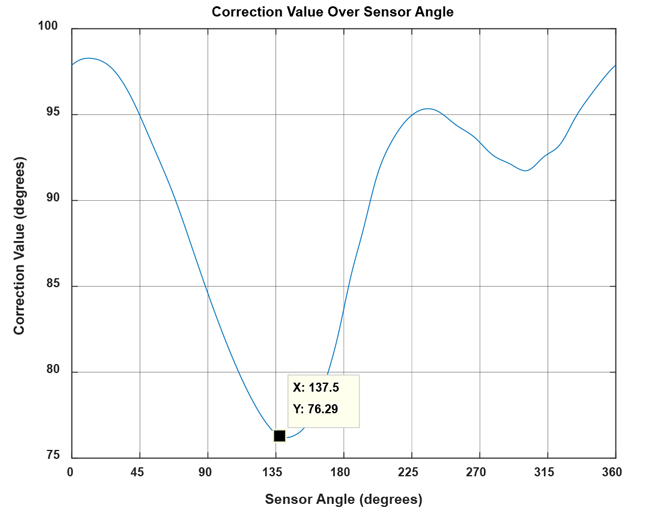
A brief check can be done to see that this curve is correct. In Table 1, it can be seen that for the sensor angle of 137.46°, the encoder angle is 213.75°. The correction curve of Figure 16 shows that at a sensor angle of 137.5°, a correction of +76.29° needs to be applied. As 137.46 + 76.26 = 213.72° ≅ 213.75°, the correction curve calculated is applicable.
At the next step, the correction curve needs to be stored in an efficient way, so that the correction value can be calculated for any input. This will be done using harmonic approximation, linear interpolation, and a lookup table.
Harmonic Approximation
Concept
Each repeating signal can be divided into its constituting frequencies.
The correction curve is repeated after every rotation, so that it can be completely described as a set of frequencies. Repeating the correction curve may make it clearer that various frequencies are contained in the correction curve.
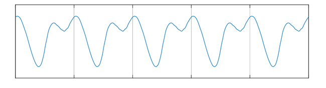
An advantage of the harmonic approximation is that the correction curve can be described with acceptable accuracy using only a few parameters. However, the calculation of cosine may be too
slow for some platforms or applications.
Implementation
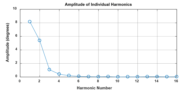
Using a Fourier transform, the phase and amplitude for each composing frequency of the correction curve can be determined. The 4096 data points of the correction curve lead to a 4096-point FFT result. However, most energy is in the lower frequencies. Below, only the offset value and the first 16 harmonics of the correction curve are extracted:
This yields an offset correction of 89.82°, and the following amplitudes of the harmonics:%% Fourier transform the correction, discarding the values after the 16th
% and scaling energy by length of the table
fft_table = fft(correction_curve)/length(intermediategrid);
offset_correction = abs(fft_table(1));
correction_pha = angle(fft_table(2:17));
correction_amp = 2*abs(fft_table(2:17));
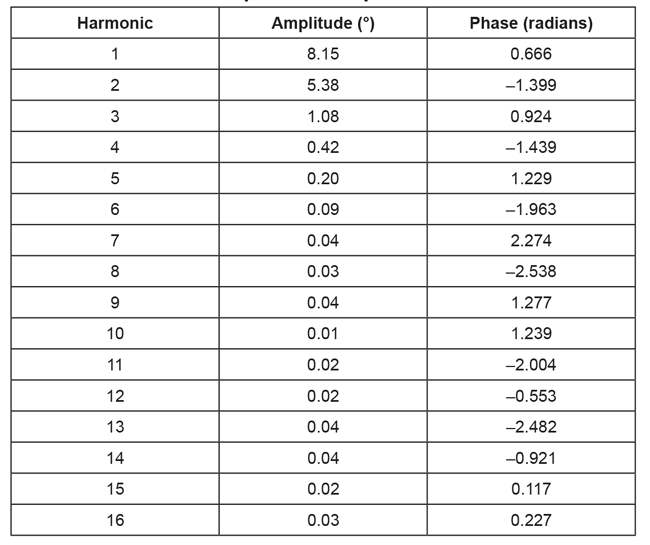
The complete result table up to the 16th harmonic is found below:
Table 3: Harmonics amplitude and phase data
Application
The correction value for the nth harmonic at a specific angle can be found as:
corr(n) = correction_amp(n)× cos[n × sensor_angle + correction_pha(n)],
where the 0th harmonic is offset correction and should be taken into account as well. Practically applied, the following code results in four harmonics. As the cosine function expects radians
as input, the angle values are converted to radians. The correctionamplitude stored in the table is in degrees, since the input to the Fourier transform was in degrees.
%% apply harmonic correction for four harmonics
restored_signal_4_harmonics = mod(sensor_data + (...
offset_correction + ...
correction_amp(1)*cos(1*(sensor_data/360*2*pi) + correction_pha(1)) + ...
correction_amp(2)*cos(2*(sensor_data/360*2*pi) + correction_pha(2)) + ...
correction_amp(3)*cos(3*(sensor_data/360*2*pi) + correction_pha(3)) + ...
correction_amp(4)*cos(4*(sensor_data/360*2*pi) + correction_pha(4)) ...
),360);
This code performs the correction for all the sensor angles in sensor_data.
Implementation of this correction in a loop will reduce code size for microcontroller implementations, but was not used here for code clarity reasons.
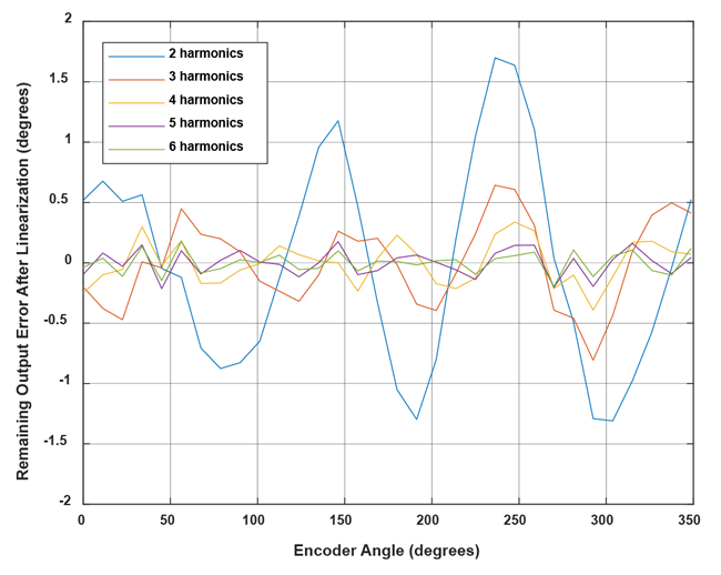
Figure 19 shows the remaining output inaccuracy after linearization over the 16 recorded angles from Table 1. The remaining error decreases by adding more harmonics. When choosing which harmonic to compensate, it is best to choose the harmonics in order of decreasing amplitude. For example, if harmonic 1, 2, and 4 have a large amplitude, while harmonic 3 has a smaller amplitude, then correcting harmonic 1, 2, and 4 will give a better result than correcting harmonic 1, 2 and 3.
Linear Interpolation
Concept
The correction curve can be approximated by a piecewise linear function. For this function, it is required to store support points as pairs of sensor coordinates and correction values.
In Figure 8, these pairs would be [(y'0, c0,) … (y'n, cn)]. Between the support points, linear interpolation is performed. In angle sensor linearization applications, it is useful to use an equidistant grid of sensor angles. In this way, the sensor angle values [y'0 … y'n] do not need to be stored, and the implementation of the linear correction becomes easier. For example, it is possible to store 32 correction values, which will then be applied at sensor angles of 0°, 11.25°, 22.50°, etc.
The points to be stored can be determined by different criteria.
The simplest way to determine them is by choosing points on the correction curve at said sensor angles, which will be referred to as “on-curve” linear interpolation. However, the points can also be optimized for a least-squares error of the stored correction curve. This will be referred to as “least-squares” linear interpolation. Other optimization strategies are possible, but will not be
described in this document.
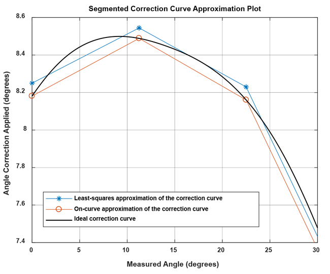
linear interpolation with parameters determined by
on-curve and least-squares method
The least-squares method reduces the amount of storage parameters needed by about 50% for the same maximum error and is less sensitive to single measurement outliers. Therefore, the leastsquares method will be used here to determine the linear interpolation support points.
Implementation
The correction curve needs to be approximated using a piecewise linear function. Because the support point should be chosen in a least-squares error fashion, the data before and after the support
point also contributes in determining its final value.
This creates a problem for the first and last point. The first support point at 0° only has a correction curve to the right side of the point, so that the data close to 360° would not be taken into account. To avoid this problem, the correction curve will be repeated three times, and a piecewise linear least-squares approximation of that curve will be calculated. Then, only the central part will be used to choose the parameters used. This concept is shown in Figure 21.
Fit Calculation
The code to replicate the correction curve and calculate the fit is given below:
%% piecewise linear approximation of the correction curve
lin_sup_nodes = 32;
% repeat the correction table three times to avoid
% corner effects on correction calculation.
triple_correction_curve = repmat(correction_curve,3,1);
triple_correction_curve(end+1) = triple_correction_curve(1);
% do the same with the angle input
triple_output_grid = 0:(360/4096):(3*360);
% calculate support points
XI_lin_triple = linspace(0,3*360,lin_sup_nodes*3+1);
YI_lin_triple = lsq_lut_piecewise( triple_output_grid(:), ...
triple_correction_curve, XI_lin_triple );
% use only the central points to calculate the correction:
YI_lin = YI_lin_triple(lin_sup_nodes+1 : 2*lin_sup_nodes+1);
XI_lin = linspace(0,360,lin_sup_nodes+1);
The lsq_lut_piecewise function is reprinted in Appendix A.
The list of correction parameters for 32-point linear interpolation is found below:
Table 4: Linear interpolation parameters
Note that a value for 360° was also added, even though it is identical to the one for 0°. This is needed to make correction of angles between 348.75° and 360° possible without using tricks.
Application
In MATLAB, the application of the correction is straightforward using the built-in 1D interpolation function:
The same function can also be implemented as follows to demonstrate how the calculation can be performed in a microcontroller:%% perform linear interpolation
restored_linear_signal = mod(sensor_data(:) + ...
interp1(XI_lin,YI_lin,sensor_data(:),’linear’),360);
%% perform linear interpolation manually
restored_linear_signal_man = zeros(length(sensor_data),1);
lin_sup_res = 360/lin_sup_nodes;
for i = 1:length(sensor_data)
% get index of table entry before the sensor angle
baseangle_idx = floor(sensor_data(i)/lin_sup_res);
baseangle = baseangle_idx*lin_sup_res;
% get number of degrees that we are past the table entry
offsetangle = sensor_data(i) - baseangle;
% correction is base +
correctionval = YI_lin(baseangle_idx+1) + ...
((YI_lin(baseangle_idx+2) - ...
YI_lin(baseangle_idx+1)) * offsetangle/lin_sup_res);
restored_linear_signal_man(i) = mod(sensor_data(i) + ...
correctionval,360);
end
This code performs the correction for all the sensor angles in sensor_data.
In a microcontroller implementation, efficient use of bit shifting and bit masking can remove the need for division operations. The modulo operation can be replaced by the deliberate use of integer overflows. However, subtraction, addition, and multiplication are still required.
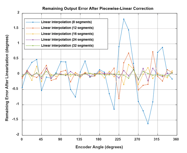
The remaining output inaccuracy after linearization for our example is shown below over the 16 recorded angles. The remaining error decreases by adding more linearization points.
Lookup Table
Concept
For linear interpolation of the correction curve, it is required to interpolate between the support points. This requires some mathematical operations, which may often take too long.
Instead of interpolating between two supporting values, it is possible to use the closest correction value directly. This method is referred to as a lookup table in this document.
The correction value for each set of angles, or bin, will be chosen as the average of the correction curve values inside that bin. This will ensure the lowest resulting RMS error of the correction curve
representation. Other strategies, such as choosing the average between the minimum and maximum correction of the respective bin, are possible, but will not be used in this document.
Using a lookup table requires storing a large number of values to reach acceptable performance. About 256 values are typically needed. The number of values does not need to be a power of two; however, microcontroller implementations in fixed-point code will benefit from using powers of two for the number of table entries.
Implementation
At first, the bin boundaries need to be defined. Then, the average of the correction curve values inside that boundary can be determined.
%% look-up table approximation of the correction curve
number_table_entries = 64;
% choose bin boundaries
XI_binlimits = linspace(0,360,number_table_entries+1);
% find average of point for each bin using function bin_lut:
YI_lut = bin_mean( ordered_output_grid(:), ...
correction_curve(:), XI_binlimits(:) );
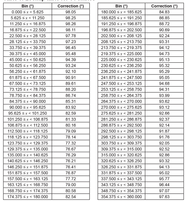
The function bin_lut is printed in Appendix B. It should be noted that correction curve values that are exactly on the boundary between two bins are included in the average of the bin for the larger values, and are excluded from the bin for the smaller values.
For example, with 64 entries, the correction curve data at an angle of 180° are used for the value of the bin 180° … 185.625°, and are not used for the bin 174.375° … 180°.
An exemplary resulting correction curve for 64 table entries is seen in Figure 23.
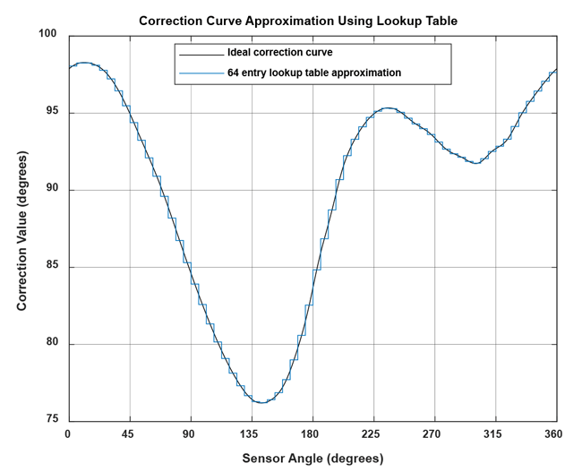
of the correction curve using 64 bins
The resulting table for 64 entries can be found in Table 5.
Table 5: Lookup table for 64 entries
Application
In MATLAB, the application of the correction is straightforward using the built-in 1D interpolation function previous-neighbor value:
restored_lut_signal = mod(sensor_data(:) + ...
interp1(XI_binlimits(1:end-1), ...
YI_lut, sensor_data(:),'previous','extrap'),360);
The same function can also be implemented as follows to demonstrate
how the calculation can be performed in a microcontroller:
number_table_entries = 64;
restored_lut_signal_man = zeros(length(sensor_data),1);
table_res = 360/number_table_entries;
for i = 1:length(sensor_data)
% get index of table entry before the sensor angle
baseangle_idx = floor(sensor_data(i)/table_res);
correctionval = YI_lut(baseangle_idx+1);
restored_lut_signal_man(i) = mod(sensor_data(i) + ...
correctionval,360);
end
This code performs the correction for all the sensor angles in sensor_data.
In a microcontroller implementation, efficient use of bit shifting and bit masking can remove the need for division operations. The angle can be used to directly index the table entry after bit shifting or masking. The modulo operation can be replaced by the deliberate use of integer overflows. Only an addition is still required.
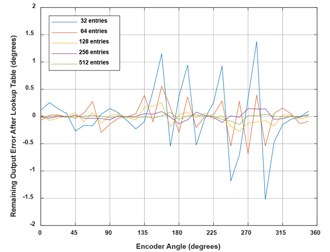
The remaining output inaccuracy after linearization for our example is shown below over the 16 recorded angles. The remaining error decreases by adding more lookup table entries.
Performance Comparison
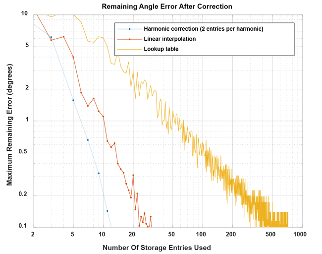
To compare the performance of the three methods explained in this document, the difference between the ideal correction curve and the representation using the three discussed methods was analyzed.
This was done using the correction curve from Figure 16. Other curves will give different results.
In on-axis applications where the required corrections are small, the number of entries used could be reduced.
To compare the storage needs of the methods, it was assumed that one storage entry is needed for each value stored for the lookup table and linear interpolation.
For harmonic linearization, two storage entries (phase and amplitude) are needed per harmonic, and a DC offset needs to be stored as well. This brings the amount of storage entries for n harmonics
to 2 × n + 1.
For harmonic correction, the harmonics applied were chosen in order of decreasing amplitude. This means, for example, that correction of the 9th harmonic (amplitude of 0.0429°) was added before adding correction for the 7th and 8th harmonics (amplitudes of 0.0361 and 0.0257°, respectively). For side-shaft applications, it is common that the 2nd and 4th harmonic are much stronger than the others. In such a case, only correcting these two may be useful.
The maximum absolute error over a full rotation was determined and plotted over storage requirements in Figure 25.
Conclusion
This document details three possible methods to linearize angular sensor data using a microcontroller. The implementations cover a wide range of memory and processing time requirements.
Contact an Allegro representative for any remaining questions or support.
APPENDIX A: FUNCTION LSQ_LUT_PIECEWISE
From https://uk.mathworks.com/matlabcentral/fileexchange/40913-piecewise-linear-least-square-fit.
Copyright (c) 2013, Guido Albertin
All rights reserved.
Redistribution and use in source and binary forms, with or without modification, are permitted provided that the following conditions are met:
* Redistributions of source code must retain the above copyright notice, this list of conditions and the following disclaimer.
* Redistributions in binary form must reproduce the above copyright notice, this list of conditions and the following disclaimer in the documentation and/or other materials provided with the distribution
THIS SOFTWARE IS PROVIDED BY THE COPYRIGHT HOLDERS AND CONTRIBUTORS “AS IS” AND ANY EXPRESS OR IMPLIED WARRANTIES, INCLUDING, BUT NOT LIMITED TO, THE IMPLIED WARRANTIES OF MERCHANTABILITY AND FITNESS FOR A PARTICULAR PURPOSE ARE DISCLAIMED. IN NO EVENT SHALL THE COPYRIGHT OWNER OR CONTRIBUTORS BE LIABLE FOR ANY DIRECT, INDIRECT, INCIDENTAL, SPECIAL, EXEMPLARY, OR CONSEQUENTIAL DAMAGES (INCLUDING, BUT NOT LIMITED TO, PROCUREMENT OF SUBSTITUTE GOODS OR SERVICES; LOSS OF USE, DATA, OR PROFITS; OR BUSINESS INTERRUPTION) HOWEVER CAUSED AND ON ANY THEORY OF LIABILITY, WHETHER IN CONTRACT, STRICT LIABILITY, OR TORT (INCLUDING NEGLIGENCE OR OTHERWISE) ARISING IN ANY WAY OUT OF THE USE OF THIS SOFTWARE, EVEN IF ADVISED OF THE POSSIBILITY OF SUCH DAMAGE.
function [ YI ] = lsq_lut_piecewise( x, y, XI )
% LSQ_LUT_PIECEWISE Piecewise linear interpolation for 1-D interpolation (table lookup)
% YI = lsq_lut_piecewise( x, y, XI ) obtain optimal (least-square sense)
% vector to be used with linear interpolation routine.
% The target is finding Y given X the minimization of function
% f = |y-interp1(XI,YI,x)|^2
%
% INPUT
% x measured data vector
% y measured data vector
% XI break points of 1-D table
%
% OUTPUT
% YI interpolation points of 1-D table
% y = interp1(XI,YI,x)
%
if size(x,2) ~= 1
error('Vector x must have dimension n x 1.');
elseif size(y,2) ~= 1
error('Vector y must have dimension n x 1.');
elseif size(x,1) ~= size(x,1)
error('Vector x and y must have dimension n x 1.');
end
% matrix defined by x measurements
A = sparse([]);
% vector for y measurements
Y = [];
for j=2:length(XI)
% get index of points in bin [XI(j-1) XI(j)]
ix = x>=XI(j-1) & x<XI(j);
% check if we have data points in bin
if ~any(ix)
warning(sprintf('Bin [%f %f] has no data points, check estimation.
Please re-define X vector accordingly.',XI(j-1),XI(j)));
end
% get x and y data subset
x_ = x(ix);
y_ = y(ix);
% create temporary matrix to be added to A
tmp = [(( -x_+XI(j-1) ) / ( XI(j)-XI(j-1) ) + 1) (( x_-XI(j-1) ) / ( XI(j)-XI(j-1) ))];
% build matrix of measurement with constraints
[m1,n1]=size(A);
[m2,n2]=size(tmp);
A = [[A zeros(m1,n2-1)];[zeros(m2,n1-1) tmp]];
% concatenate y measurements of bin
Y = [Y; y_];
end
% obtain least-squares Y estimation
YI=A\Y;
APPENDIX B: FUNCTION BIN_MEAN
Copyright (c) 2018, Dominik Geisler, Allegro MicroSystems Germany GmbHvAll rights reserved.
Redistribution and use in source and binary forms, with or without modification, are permitted provided that the following conditions are met:
* Redistributions of source code must retain the above copyright notice, this list of conditions and the following disclaimer.
* Redistributions in binary form must reproduce the above copyright notice, this list of conditions and the following disclaimer in the documentation and/or other materials provided with the distribution
THIS SOFTWARE IS PROVIDED BY THE COPYRIGHT HOLDERS AND CONTRIBUTORS “AS IS” AND ANY EXPRESS OR IMPLIED WARRANTIES, INCLUDING, BUT NOT LIMITED TO, THE IMPLIED WARRANTIES OF MERCHANTABILITY AND FITNESS FOR A PARTICULAR PURPOSE ARE DISCLAIMED. IN NO EVENT SHALL THE COPYRIGHT OWNER OR CONTRIBUTORS BE LIABLE FOR ANY DIRECT, INDIRECT, INCIDENTAL, SPECIAL, EXEMPLARY, OR CONSEQUENTIAL DAMAGES (INCLUDING, BUT NOT LIMITED TO, PROCUREMENT OF SUBSTITUTE GOODS OR SERVICES; LOSS OF USE, DATA, OR PROFITS; OR BUSINESS INTERRUPTION) HOWEVER CAUSED AND ON ANY THEORY OF LIABILITY, WHETHER IN CONTRACT, STRICT LIABILITY, OR TORT (INCLUDING NEGLIGENCE OR OTHERWISE) ARISING IN ANY WAY OUT OF THE USE OF THIS SOFTWARE, EVEN IF ADVISED OF THE POSSIBILITY OF SUCH DAMAGE.
function [ YI ] = bin_mean( x, y, XI )
% BIN_LUT bin lookup table for 1-D interpolation (table lookup)
% YI = lsq_lut_piecewise( x, y, XI ) obtains optimal (least-square sense) bin
% values for a nearest-neighbour look-up table between bin boundaries defined in XI.
if ((size(x,1) ~= 1) && (size(x,2) ~= 1))
error('Vector x must have dimension n x 1 or 1 x n');
elseif ((size(y,1) ~= 1) && (size(y,2) ~= 1))
error('Vector y must have dimension n x 1 or 1 x n');
elseif length(x) ~= length(y)
error('Vector x and y must have the same length');
end
YI = zeros((length(XI)-1),1);
for j=1:(length(XI)-1)
YI(j) = mean( y( (x>=XI(j)) & (x<XI(j+1)) ) );
end
APPENDIX C: FUNCTION ENTIRE SCRIPT USED IN THIS APPLICATION NOTE
Copyright (c) 2018, Dominik Geisler, Allegro MicroSystems Germany GmbH All rights reserved.
Redistribution and use in source and binary forms, with or without modification, are permitted provided that the following conditions are met:
* Redistributions of source code must retain the above copyright notice, this list of conditions and the following disclaimer.
* Redistributions in binary form must reproduce the above copyright notice, this list of conditions and the following disclaimer in the documentation and/or other materials provided with the distribution
THIS SOFTWARE IS PROVIDED BY THE COPYRIGHT HOLDERS AND CONTRIBUTORS “AS IS” AND ANY EXPRESS OR IMPLIED WARRANTIES, INCLUDING, BUT NOT LIMITED TO, THE IMPLIED WARRANTIES OF MERCHANTABILITY AND FITNESS FOR A PARTICULAR PURPOSE ARE DISCLAIMED. IN NO EVENT SHALL THE COPYRIGHT OWNER OR CONTRIBUTORS BE LIABLE FOR ANY DIRECT, INDIRECT, INCIDENTAL, SPECIAL, EXEMPLARY, OR CONSEQUENTIAL DAMAGES (INCLUDING, BUT NOT LIMITED TO, PROCUREMENT OF SUBSTITUTE GOODS OR SERVICES; LOSS OF USE, DATA, OR PROFITS; OR BUSINESS INTERRUPTION) HOWEVER CAUSED AND ON ANY THEORY OF LIABILITY, WHETHER IN CONTRACT, STRICT LIABILITY, OR TORT (INCLUDING NEGLIGENCE OR OTHERWISE) ARISING IN ANY WAY OUT OF THE USE OF THIS SOFTWARE, EVEN IF ADVISED OF THE POSSIBILITY OF SUCH DAMAGE.
%% sensor data definition
angle_input = [0:11.25:348.75];
sensor_data = [266.31 278.61 290.39 301.99 312.45 323.00 332.75 342.69 352.79 3.16
14.24 26.02 38.94 52.91 67.15 82.18 97.12 111.45 124.98 137.46 148.62 158.82
167.96 176.48 184.48 192.92 201.27 210.50 220.43 230.98 242.31 254.36];
%% Check rising reference angle
if any(angle_input<0) || any(angle_input>360) || any(diff(angle_input)<=0)
error('reference angle must be monotonuously rising between 0 and 360');
end
%% Check correct sensor angle range
if any(sensor_data<0) || any(sensor_data>360)
error('sensor angle must be between 0 and 360');
end
%% preprocessing
sensor_data_2 = sensor_data(:);
angle_input = angle_input(:);
% check if rising continuously with at most one overflow
if any(diff(sensor_data_2) == 0)
error('sensor data must be monotonously increasing')
elseif sum(diff(sensor_data_2) < 0 ) <= 1
% rising angle data with zero or one overflow, overflow will be corrected
sensor_data_2 = sensor_data_2(:) + 360*cumsum([false; diff(sensor_data_2(:)) < 0 ]);
elseif sum(diff(sensor_data_2) < 0 ) > 1
error('only one data decrease permitted as overflow')
end
% correctly wrap around sensor data
rollovercorrection = round((mean(sensor_data_2) - 180)/360) * 360;
sensor_data_2 = sensor_data_2 - rollovercorrection;
% extend sensor data
sensor_data_ext = [sensor_data_2(:); sensor_data_2(:)+360; ...
sensor_data_2(:)+720];
% extend input data
angle_input_ext = [angle_input(:); angle_input(:)+360; ...
angle_input(:)+720];
%% plot magnet measurements after preprocessing finished
figure;plot([angle_input(:)],[sensor_data_2(:)],'o-');
xlabel('Encoder angle [deg]');
ylabel('Output angle [deg]');
grid on;
xlim([0 360]);
title({'Output field direction over encoder direction'});
%% use spline to move the data from an ordered input grid
% onto an ordered output grid:
ordered_output_grid = 0:(360/4096):(360-360/4096);
intermediategrid = ordered_output_grid + 360;
projection = spline(sensor_data_ext, angle_input_ext, ...
intermediategrid);
    % calculate the required correction of the data:

correction_curve = projection - intermediategrid;

correction_curve = correction_curve(:);
%% Fourier transform the correction, discarding the values after the 16th
% and scaling energy by length of the table
Allegro MicroSystems, LLC 20
955 Perimeter Road
Manchester, NH 03103-3353 U.S.A.
www.allegromicro.com
fft_table = fft(correction_curve)/length(ordered_output_grid);
offset_correction = abs(fft_table(1));
correction_pha = angle(fft_table(2:17));
correction_amp = 2*abs(fft_table(2:17));
    %% apply harmonic correction for four harmonics

restored_signal_4_harmonics = mod(sensor_data + (...

offset_correction + ...

correction_amp(1)*cos(1*(sensor_data/360*2*pi) + correction_pha(1)) + ...

correction_amp(2)*cos(2*(sensor_data/360*2*pi) + correction_pha(2)) + ...

correction_amp(3)*cos(3*(sensor_data/360*2*pi) + correction_pha(3)) + ...

correction_amp(4)*cos(4*(sensor_data/360*2*pi) + correction_pha(4)) ...

),360);
%% piecewise linear approximation of the correction curve

lin_sup_nodes = 32;

% repeat the correction table three times to avoid

% corner effects on correction calculation.

triple_correction_curve = repmat(correction_curve,3,1);

triple_correction_curve(end+1) = triple_correction_curve(1);

% do the same with the angle input

triple_output_grid = 0:(360/4096):(3*360);

% calculate support points

XI_lin_triple = linspace(0,3*360,lin_sup_nodes*3+1);

YI_lin_triple = lsq_lut_piecewise( triple_output_grid(:), ...

triple_correction_curve, XI_lin_triple );

% use only the central points to calculate the correction:

YI_lin = YI_lin_triple(lin_sup_nodes+1 : 2*lin_sup_nodes+1);

XI_lin = linspace(0,360,lin_sup_nodes+1);
%% perform linear interpolation
restored_linear_signal = mod(sensor_data(:) + ...
interp1(XI_lin,YI_lin,sensor_data(:),'linear'),360);
    %% perform linear interpolation manually

restored_linear_signal_man = zeros(length(sensor_data),1);

lin_sup_res = 360/lin_sup_nodes;

for i = 1:length(sensor_data)

% get index of table entry before the sensor angle

baseangle_idx = floor(sensor_data(i)/lin_sup_res);

baseangle = baseangle_idx*lin_sup_res;

% get number of degrees that we are past the table entry

offsetangle = sensor_data(i) - baseangle;

% correction is base +

correctionval = YI_lin(baseangle_idx+1) + ...

((YI_lin(baseangle_idx+2) - ...

YI_lin(baseangle_idx+1)) * offsetangle/lin_sup_res);

restored_linear_signal_man(i) = mod(sensor_data(i) + ...

correctionval,360);

end
%% perform look-up table correction
number_table_entries = 64;
% choose bin boundaries
XI_binlimits = linspace(0,360,number_table_entries+1);
% find average of point for each bin using function bin_lut:
YI_lut = bin_mean( ordered_output_grid(:), ...
correction_curve(:), XI_binlimits(:) );
%% apply look-up table linearization
    restored_lut_signal = mod(sensor_data(:) + ...

interp1(XI_binlimits(1:end-1), ...

YI_lut, sensor_data(:),'previous','extrap'),360);
%% apply look-up table linearization manually
restored_lut_signal_man = zeros(length(sensor_data),1);
table_res = 360/number_table_entries;
for i = 1:length(sensor_data)
% get index of table entry before the sensor angle
baseangle_idx = floor(sensor_data(i)/table_res);
correctionval = YI_lut(baseangle_idx+1);
restored_lut_signal_man(i) = mod(sensor_data(i) + ...
correctionval,360);
end
%% plot the remaining error after lienarization with the three methods
figure;
plot(angle_input(:),mod(180+restored_linear_signal(:)-angle_input(:),360)-180,'.-', ...
angle_input(:),mod(180+restored_signal_4_harmonics(:)-angle_input(:),360)-180,'.-', ...
angle_input(:),mod(180+restored_lut_signal(:)-angle_input(:),360)-180,'.-' ...
);
grid on;legend('Linear interpolation (32 segments)','harmonic correction (4 harmonics)',
'look-up table (64 entries)');
xlim([0 360]); xlabel('Measured angle [deg]');
ylabel('Expected error after linearization [deg]');
The information contained in this document does not constitute any representation, warranty, assurance, guaranty, or inducement by Allegro to the customer with respect to the subject matter of this document. The information being provided does not guarantee that a process based on this information will be reliable, or that Allegro has explored all of the possible failure modes. It is the customer’s responsibility to do sufficient qualification testing of the final product to insure that it is reliable and meets all design requirements.
1] Allegro Angle Position Sensor ICs, /en/Products/Magnetic-
Linear-And-Angular-Position-Sensor-ICs/Angular-Position-Sensor-ICs.aspx